
S is a language for data analysis and statistical computing. It has currently two implementations: one commercial, called S-Plus, and one free, open source implementation called R. Both have advantages and disadvantages.
S-Plus has the (initial) advantage that you can work with much of the functionality without having to know the S language: it has a large, extensively developed graphical user interface. R works by typing commands (although the R packages Rcmdr and JGR do provide graphical user interfaces). Compare typing commands with sending SMS messages: at first it seems clumsy, but when you get to speed it is fun.
Compared to working with a graphical program that requires large amounts of mouse clicks to get something done, working directly with a language has a couple of notable advantages:
Of course the disadvantage (as you may consider it right now) is that you need to learn a few new ideas.
Although S-Plus and R are both full-grown statistical computing engines, throughout this course we use R for the following reasons: (i) it is free (S-Plus may cost in the order of 10,000 USD), (ii) development and availability of novel statistical computation methods is much faster in R.
Recommended text books that deal with both R and S-Plus are e.g.:
Further useful books on R are:
To download R on a MS-Windows computer, do the following:
Instructions for installing R on a Macintosh computer are also found on CRAN. For installing R on a linux machine, you can download the R source code from CRAN, and follow the compilation and installation instructions; usually this involves the commands ./configure; make; make install. There may be binary distributions for linux distributions such as RedHat FC, or Debian unstable.
You can start an R session on a MS-Windows machine by double-clicking the R icon, or through the Start menu (Note that this is not true in the ifgi CIP pools: here you have to find the executable in the right direction on the C: drive). When you start R, you’ll see the R console with the > prompt, on which you can give commands.
Another way of starting R is when you have a data file associated with R (meaning it ends on .RData). If you click on this file, R is started and reads at start-up the data in this file, along with the command history in the .Rhistory file in the same directory.
Try this using the students.RData file, that you will find at http://ifgi.uni-muenster.de/~epebe_01/Geostatistics/students.RData. Next, try the following commands:
(Note that you can copy and paste the commands including the > to the R prompt, only if you use "paste as commands")
You can see that your R workspace now has two objects in it. You can find out which class these objects belong by
If you want to remove an object, use
If you want so safe a (modified) work space to a file, you can use the menu (windows) or:
First make sure that you finish the introductory material up to and including the chapter on Reading data from files
Import the students sample data, collected at the first lecture. Either do this by loading the R data file mentioned above, or importing the raw data in csv as explained on the course web site.
Exercise 2.1 Look at a summary of the data. Which of the variables are
nominal?
Exercise 2.2 For each of the variables, find out what the modus is, by using
function table on them.
One way to do this is to look up the maximum frequency manually. Automatic lookup is obtained as follows:
Distributions can be plotted by function hist. Execute the following two commands:
Exercise 2.3 [HAND IN] Try to explain how the results returned from the second
command relate to the plot obtained by the first and how they relate to the data.
Which of the following values can be read from the plot; give values if possible. How
many times is Weight 100kg? How many times is Weight below or equal to100kg?
Which Weight is the most frequent?
As the modus of continuous variables depends on the classification, we can use hist for this, e.g. by
Exercise 2.4 Find out what the 10 refers to by reading the help for hist, and then
compute the mode for Weight, when using 10, 20, 30, 40 and 50 classes.
Read the help for functions median and quantile
Exercise 2.5 Compute the median for each of the variables in the students data
set for which this makes sense
Compute the body-mass-index (bmi) as follows:
Exercise 2.6 Between which two values do the middel 90% of the values lie for
variables bmi and Length, in the students data set?
Exercise 2.7 Above which value of the Weight variable do we have 75% of the
observations?
Exercise 2.8 Which percentage of the bmi observations lie above 25 (overweight,
according to Wikipedia)?
(For the last question, use the transformation to logical:
and function sum.)
It seems there is an outlying value in the Weight data of students. Look at the plot given with
try to explain what you see, and point out which observation is (most) doubtful.
Compute the mean and median weight values:
As mean values depend on all observations, it is advisable to compute them from data that do not contain outliers. One approach to do this, is by removing the outlier, and continue, e.g. by
Another approach to get rid of outliers is by using trimmed means. Find out what is meant by this by reading carefully the documentation of the trim argument to function mean. Let us try:
Exercise 2.9 [HAND IN] Explain why the last two commands give the same
result.
Exercise 2.10 [HAND IN] What are the advantages and disadvantages
of both approaches: (i) manual outlier removal, (ii) computing trimmed
statistics, for obtaining mean values that are not influenced by outliers?
Exercise 2.11 What is the interquartile range for Length and Weight?
Exercise 2.12 What is the standard deviation for Weight?
Exercise 2.13 Between which two values do we find the middle 68% of the Weight
values?
Exercise 2.14 How often does the standard deviation of Weight fit in this
68%-range?
As a general hint: R under windows has the option Record plots; you will find it in the menu only when the plot window is activated (blue). Check this option and you can go to previous/next plots with PgUp/PgDown when in the plot window.
Exercise 3.1 Using function hist, plot a histogram of variable bmi in the students
data set.
The book Sachs and Hedderich suggest to use function ecdf for to compute empirical cumulative density functions, as in
Exercise 3.2 [HAND IN] Estimate visually which percentage of the data
has bmi values large than 25. As an aid, use abline to draw vertical lines.
There are different ways of drawing grouped histograms. Consider these two cases:
Exercise 3.3 [HAND IN] When the goal is to compare bmi as a function of
gender, which of the two representations do you prefer? Briefly argue why.
Consider the box-and-whisker plot obtained by
Exercise 3.4 Why are the three largest observations drawn as small circles for the
female students, but not so for the male students?
For the following exercise, consider the following plots
Exercise 3.5 The help of function hist mentions, under section See Also, that
“Typical plots with vertical bars are not histograms”. (This may be taken as a
comment towards a rather popular spreadsheet program.) What is the main
difference between bar graphs and histograms, and for what kind of data is each of
them used?
The famous sunspot data (H. Tong, 1996, Non-Linear Time Series. Clarendon Press, Oxford, p. 471.) contains a feature that is only visible when the aspect ratio of the plot is controlled well.
Exercise 3.6 [ADVANCED] What is this feature, i.e. what characteristic of these
data are visible in the lower, but not in the upper plot?
The following exercise is about the scatter plot matrix, obtained e.g. for the meuse data set (top soil heavy metal contents; from: Burrough and McDonnell, Principles of GIS, 2nd ed, OUP) by
Exercise 3.7 [HAND IN] Are the lower-left (column 1, row 4) and top-right (column
4, row 1) sub-plots in this matrix related, and if so how?
Some of the following exercises are easiest done by hand, or with a hand calculator. In absence of a hand calculator, expressions can be typed on the R prompt, try e.g.
Consider the following table, which tabulates gender agains the frequencies of passing a given test:
| Male | Female | |
| passed | ? | 80 |
| failed | 10 | 40 |
Exercise 4.1 Given that passing the test is independent from gender, what is the
expected frequency for the cell with a question mark?
Exercise 4.2 [HAND IN] Given that 10 male students passed the test in the incomplete table above, estimate the following probabilities:
In the answers, use the formal notations, such as Pr(male | pass), and the appropriate
symbols for AND and OR.
Exercise 4.3 [HAND IN] Given there are 30 female and 60 male students, give cross tables with expected frequencies of passing a test, for the case where
Now generate 6 vectors with random uniform numbers, of length 1, 10, 100, 1000, 10000 and 100000. Compute the fraction of values below 0.6 for each vector.
Exercise 4.4 [HAND IN] How do the values compare to the expected value (0.6),
and how could you explain the differences?
Exercise 4.5 When would you expect obtaining a fraction of exaclty 0.6?
Exercise 4.6 [HAND IN] Suppose you take part in a quiz. The quiz master shows
you three doors. Behind one of the three doors a price is hidden. Opening the door
with the price behind it gives you the price. You are asked to choose one door. Then,
the quiz master opens one of the remaining doors, with no price behind it. Now you
are allowed to switch your choice to the other remaining closed door. To maximize
the probability of getting the price, should you (a) choose the other door, (b) stick
with your original choice, or (c) is switching irrelevant for this probability? Explain.
The following R commands give density, distribution function, quantile function and random value generation for the binomial distribution:
is the probability to have 5 sucesses if 10 samples are drawn independently and each has a probability of sucess of 0.5 (dbinom() ist the density function).
is the probability to have up to 5 (e.g. 0 or 1 ... or 5) sucesses in the same experiment (pbinom() is the cummulative distribution function). «» = x = qbinom(p = 0.1,size = 10, prob = 0.5) is the 0.1-Quantile of the same distribution; i.e. (if the experiment is done very often) the lowest 10% of the results will have no more than x successes.
generates randomly 5 possible outcomes of the experiment (for each draw 10 times with sucess of 0.5).
There exist similar functions for other distributions, try
For all of them there are the four functions. The use of the first parameter is the same as above. The other parameters are needed to define the distribution, e.g. pnorm(q = 1, mean = 100, sd = 5) gives the values of a normal distribution with mean = 100 and standard deviation = 5.
In the following R commands, a Bernoulli sequence is generated
Generate a similar sequence using the function rbinom.
Exercise 5.1 [HAND IN] Which generating probability of success (p) has to be
used?
Exercise 5.2 Suppose we have a bowl with 25% red balls, and a single experiment
involves the sampling of 10 balls with replacement, counting the number of
red balls in the sample. Generate the outcome of 100 such experiments.
Exercise 5.3 Draw a histogram of the result.
Exercise 5.4 Repeat this for 100000 experiments, and draw a histogram of the
result. Why are there empty bars in this graph?
With the command
you plot the probabilities for all the outcomes.
Exercise 5.5 Create a similar plot for all the probabilities when when the
experiment uses the same bowl, but draws 100 instead of 10 balls independently.
Exercise 5.6 Check that the latter probabilities sum to exactly one.
Suppose we are interested in the occurence pattern of the Green tiger beetle, in our study site of 2 km × 3 km. The hypothesis is that per square meter on average 0.05 of such beetles live. We have plots of 3 × 3 meter, and assume that we do catch all beetles in such a plot during an experiment.
For a normal distribution with mean 10 and standard deviation 1, the probability of having a value below 12 is found by
Exercise 5.7 [HAND IN] Assuming that body length of the students data set is
normally distributed, and assuming that the sample mean and standard deviation are
the true values, What is the probability of having a student with length larger than
195 cm?
Exercise 5.8 Which of the distributions are discrete / continuous: binomial
distribution, Poisson distribution, uniform distribution, normal distribution, Gaussian
distribution?
Imagine a multiple choice test with 40 questions, each having 4 answers whereof 1 is correct. To pass the test you need 20 correct answers. For the following exercises give the R command and the value(s). If you can not find the command, give the distribution and value (e.g. normal distribution, mean = 9, sd = 4, density in x = 2).
Exercise 5.9 You did not prepare and rely on guessing. How could you use R to
give random answers?
Exercise 5.10 If you guess all answers, what is the probability that you fail?
(What kind of experiment is it, how are the parameters?)
Exercise 5.11 The time students need is approximately normally distributed with
mean 60 minutes and standard deviation 10 minutes. After how much time will 90%
of the students have finished?
Exercise 5.12 [HAND IN] Create a normal probability plot for the variable bmi in the students data set. Add the line that indicates a reference normal distribution.
Can we consider bmi as approximately normally distributed? What are the mean
and standard deviation (do not calculate but describe how to tell from the
plot).
Load the http://www.ai-geostats.org/index.php?id=45SIC97 data, imported to an R file, from http://ifgi.uni-muenster.de/~epebe_01/Geostatistics/sic97.RData to your working directory. Start R by double-clicking the icon of the downloaded file.
Show the data, using
(Note that sp needs to be loaded, otherwise the correct method for imaging spatial grids is not available.)
The area shown is a digital terrain model, projected in some lambert projection system (with undocumented offset). As an alternative, you might use
which takes longer and shows a scale bar on the side.
To plots generated by image it is however easier to add information incrementally:
We will consider this DTM to be the target population. Compute it’s mean, variance and standard deviation, and write them down:
Exercise 6.13 [HAND IN] How do we compute the standard error for the mean,
when we take a simple random sample of 10 observations? Write down the equation
used and the value found.
We can take a simple random sample of size 10:
Exercise 6.14 [HAND IN] compute the 95% confidence interval for the population
mean, based on this sample of 10 observations, using the true (population) variance;
give both the equation and the answer.
Look at the range and the distribution form of the altitude data:
Exercise 6.15 [HAND IN] Describe the range and form of the distribution, and
explain what you see (this should be an easy question).
Now we are going to do draw 100 samples of size 3 each, and compute their mean
Do the same thing for samples of size 10, and 100.
Exercise 6.16 [HAND IN] (i) How does the range of the distribution change when
the sample size becomes larger? Explain this phenomenon, and give a general
equation for a measure of spread for the simple random sample means of a given
sample size. (ii) How does the distribution change when sample size increases?
Exercise 6.17 [HAND IN] Repeat the above procedure, instead of simple random
sampling now use (i) regular sampling, (ii) stratified sampling and (iii) systematically
unaligned sampling. How does the range and standard deviation of the means
obtained change, compared to simple random sampling? Try to explain why this is
the case.
Load the pm10 data file pm10.txt from the course web site. If needed, set path (setwd) to the place where you save the file, and read file (the header contains the names of the monitoring stations (VMUE, VMSS) and must therefore be read seperately, set: header=TRUE)
The data are the weights of respirable dust particles (below 10 μm) in mg/m3 air from two monitoring stations in Münster (Steinfurter Straße: VMSS, Friesenring: VMUE) measured during winter 2006/07. The measured values are averages over consecutive periods of 30 min. Days with missing or negative data have been omitted.
The whole dataset VMUE shall be the population. We know the standard deviation σ. Calculate it and call it sVMUE.
Exercise 7.1 Compute the standard error for the estimator of the mean for a
sample size of 50 and call it seVMUE50.
Draw a random sample of size 50 from VMUE:
(Explain what VMUE50 is by looking at its construction, and repeating it.)
Exercise 7.2 [HAND IN] Calculate from this random sample
Compare the intervals, explain the differences.
Exercise 7.3 Calculate with σ and the random sample the values
Write down the onesided confidence intervals and compare with the twosided confidence
intervals.
Draw a random sample of size 5 from VMSS, and call it VMSS5. Calculate from this random sample mean (=mVMSS5) and sample standard deviation (s=sVMSS5).
Exercise 7.4 [HAND IN] Calculate with the method described in the lecture:
What is the difference from calculating confidence intervals using σ?
Hint: for the 90% confidence interval, use
Look for the required values in the results from
Exercise 7.5 [HAND IN] You want to know the population mean from a sample.
The 95% confidence interval has to be smaller than 20 (i.e. you do not want to
underestimate the mean by more than ten and not to overestimate it by more than
ten, with probability 0.95). How big must the size of the sample be? (This
can be calculated directly or by trying it out. Note you do not need the
mean but only the population standard deviation sVMSS for the calculation.)
Draw random samples of size 100 from both columns (see 7.1), and save them to vectors with names VMUE100 and VMSS100
Do a t-test for the difference of the means of VMUE and VMSS (mVMUE-mVMSS) based on those samples
Exercise 7.6 Can you be 95% confident that the population means mVMUE,
mVMSS are different (short explanation)?
Draw samples
a)
b)
Exercise 7.7 What is the difference?
Exercise 7.8 Give the 95% confidence interval for the difference of the means with
the data from b).
Exercise 7.9 Do a paired t-test, give the 95% confidence interval for the mean of
the differences. See hint below;
Exercise 7.10 [HAND IN]Remember the data are measurements from two stations,
each column belongs to a station, each row to a date. What happens in 7.8 compared
to 7.9? Which method tells you more about the difference between the two stations
at one time?
Load the student data set and try:
Exercise 8.1 [HAND IN] Test, for the students data set, whether the bmi for
students depends on gender, assuming equal variance of both groups. Write out the
first 4 steps of the formal procedure (hypothesis testing), and use the p value to find
the conclusion.
Exercise 8.2 [HAND IN] Explain in your own words what the p-value of the test
result mean, and how it is related to the t value.
Exercise 8.3 [HAND IN] Test, for the students data set, whether the bmi for male
students is equal to 25. Use the t-value and follow the 7 steps of formal testing.
Compare your results to those obtained by using the function t.test for this.
Exercise 8.4 Test, for the students data set, whether the bmi for male students
exceeds 25
Exercise 8.5 Test, for the students data set, whether the bmi for male students is
smaller than 25
Exercise 8.6 Can you do a paired t-test to compare bmi for male and female
students? If yes, show how. If no, explain.
Exercise 8.7 [HAND IN] Explain how in the first and third exercise of this section
the t value is calculated; give also details how in both cases the standard error of
mean in the denominator is calculated
Work with the students data set, and try the following:
Exercise 9.1 [HAND IN] Assume that the groups have equal size, and that
the variance of both groups is equal. How large a sample size would result
in a confidence interval half as wide? (Hint: this is easiest done by hand)
Do the t computation of the example above step by step:
and check that the final value equals t.
Exercise 9.2 [HAND IN] Describe in words what v is.
The function power.t.test can compute the power, delta (difference of alternative means) or required sample size for a test if all other parameters are given:
Computes the minimal distance of alternative hypotheses (delta) which can be destinguished by a test at significance level 0.05 and with power 0.95 if sample size is 10 and standard deviation of the data is 1. This can also be computed for one-sided tests with alternative = "one.sided" and for other test types (type = "one.sample", type = "paired").
Exercise 9.3 [HAND IN] Compute the power of the test above: use the square-root
of v as sd and delta = m1 - m2, set the correct sample size (see NOTE). You can
use the default test type and alternative.
Exercise 9.4 Which sample size would have been required to obtain a power of at
least 0.95, and of at least 0.9? (Note that sample size cannot be a broken number)
Exercise 9.5 [HAND IN] Does factor Year have a significant effect on
Weight(please hand in the ANOVA output)?
Exercise 9.6 [HAND IN] Explain how F got computed from the data, and what
the Pr value means
A balanced sample from the students dataset is given by
and compare the ANOVA models
Exercise 9.7 Why does significance of I.am. change between the models? (Explain
how F got computed in each case.)
Consider the meuse data set.
The heavy metal concentrations are thought to originate from sediment, deposited by the Meuse river, and the near-river soil samples clearly contain higher heavy metal concentrations. Also the concentrations of the different heavy metals are correlated.
Plot the heavy metal concentrations against each other.
Exercise 10.8 [HAND IN] Try to tell which metals are strongest and which are
weakest correlated. Compute these two correlations. Test, if the smaller one is still
significant (see lecture for command; give the command and a concluding sentence).
Do a linear regression of zinc on dist:
Exercise 10.9 [HAND IN] Describe in your own words what the residual standard
error is, and how it is computed.
Plot the data and fitted line:
Exercise 10.10 The plot shown contains the least-squares line of zinc as a linear
function of dist, distance to river. Comment on whether this model is useful to
predict zinc concentrations in the area.
Hint: also look at the predicted values (regression line values) for the data points, as in
An alternative is to look at the same pair of variables, but to transform the dependent variable, e.g. by taking the logarithm:
Exercise 10.11 [HAND IN] Is this model better, worse or of equal value compared
to the first, when we consider how realistic the fitted, or predicted values are?
Exercise 10.12 [HAND IN] Write down the regression equation for the fitted values of log zinc, with the estimated values for the regression coefficients, as in
but then with a and b replaced with their estimated values.
Exercise 10.13 Use the regression equation from above to compute the modelled
log(zinc) value for zinc where dist = 0.3. You may compare it with the results
from predict
Exercise 10.14 What is the modelled value of zinc for dist = 0.3?
Exercise 10.15 [HAND IN] Compute a 95% confidence interval for the
regression slope in this last regression model, either by hand or with R.
This is a regression completely done by hand, you may use a calculator or
R.
Consider the following data (Wonnacott & Wonnacott p. 358),
| X fertilizer | Y yield |
| (lb/acre) | (bu/acre) |
| 100 | 40 |
| 200 | 50 |
| 300 | 50 |
| 400 | 70 |
| 500 | 65 |
| 600 | 65 |
| 700 | 80 |
Exercise 11.1 Plot the data by hand or by R. Copy the plot as a bitmap (.bmp)
and add by hand the regression line, remember the residuals (vertical distance from
points to line) should be minimal.
Exercise 11.2 To calculate the regression coefficients use the formulas (see lecture)
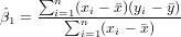
and

You may do that completely by hand, filling the following table
| Data | Deviation | Products | ||||
| X | Y | x = X - | y = Y - | xy | x2 | |
| 100 | 40 | -300 | -20 | 6000 | 90000 | |
 |  |  |  |  |  |
|
| ∑ |  = 400 = 400 |  = = | ∑ x = 0 | ∑ y = 0 | ∑ xy = | ∑ x2 = |
Exercise 11.3 [HAND IN] Write the regression equation, using the regression
coefficients calculated in the last exercises or by R.
Exercise 11.4 Plot the regression line (by hand or by R).
Exercise 11.5 [HAND IN] Which yield would you expect if using 250 lb fertilizer
per acre?
Load the students dataset into the path.
Turn Gender into a numeric dummy variable (female: 0, male: 1)
We want to do regression of Weight by Length and to include Gender if convenient. First have a look at the data
Exercise 11.6 Copy the plot as a bitmap and add a regression line (in black) by eye.
Imagine you would do regression on males and females separately and add a coloured
regression line for each.
Build three models.
Exercise 11.7 [HAND IN] Complete the following table
| Model | general Form | regression formula | Ra2 |
| lm.L | Y = β0 + β1X1 | Weight = -120 + 1.1 * Length | 0.4649 |
| lm.LaG | Y = β0 + β1X1 + β2X2 | ||
| lm.LiG | Y = β0 + β1X1 + β2X2 + β3X1x3 |
Save the coefficients
Exercise 11.8 [HAND IN] Consider the second model lm.LaG and the third model
lm.LiG. Each of them can be split into a model for female and a model for male
(Gender is 0 or 1). Give for each of the models the equation for males and females.
Plot the models (male and female in colors)
(Hint: in R open one plot then set "History" to "record" then you can switch between
plots by "page up" and "page down".)
Exercise 11.9 [HAND IN] What do the models describe? (assign models to the
descriptions below if they fit)
Exercise 11.10 What is the true influence of only Length on Weight? Which of the
models is best?
Exercise 11.11 [HAND IN] Are all parameters in all models significant at the 5%
level? If not, does it make sense to keep them anyway?
Carefully read the help of predict.lm, the predict method that applies to objects of class lm, e.g. by the command ?predict.lm.
Load the data
Compare the linear and quadratic models of log-zinc with distance to river in the meuse data set:
Exercise 12.1 What is given by predict(lm(zinc ˜ dist, meuse),
new)?
Add more regression lines
(Set "History" to "record", you will need plots several times to add something.)
Exercise 12.2 Discuss the advantages and disadvantages of using a linear (lm1), a
quadratic function in dist (lm2), or a quadratic function in square-root of distance
(lm3). How realistic are the predictions?
Compare also the following two models for transformed data:
They can be plotted to the original scale, with a little bit work (go back to the plot of the above models or start again plotting the values by plot(zinc ˜ dist, meuse)):
Exercise 12.3 [HAND IN] Which of the 5 models (lm1, ..., lm5) do you prefer,
why?
Suppose that one of the observed values is zero, as in
we try to do regression on the logarithm of these values:
Exercise 12.4 [HAND IN] Why does this fail?
(Prediction is found at W&W p. 384-386)
Predicting values can be done under all circumstances, defined by the values of the X-variables, or predictors.
One particular case, common to geostatistics, is that where the X-variables come as maps. In the models defined in 12.1, dist and zinc vary in space
Therefore the models give a prediction for each point in space.
Exercise 12.5 [HAND IN] Why are there high values (yellow) far away from the
river in the lzn.pred2 plot? Why are the contours in the lzn.pred5 plot closer for
high values at the river than for low values far away?
Now we continue with only lm5 on the transformed data.
Exercise 12.6 [HAND IN] There is some uncertainty in estimating the parameters of
the line. Copy the plot as a bitmap and add some other possible regression
lines. For which X values we know best where the regression line should
be?
The model can calculate uncertainties (here for the first point)
The values are related
Exercise 12.7 Why is the result always = 1?
Add confidence intervals for the means to the plot:
Exercise 12.8 [HAND IN] explain in words what the intervals between each pair of
blue minus symbols represent.
Plot the standard errors as a map
Exercise 12.9 Why are the lowest standard error values not found near to or far
from the river, but somewhere in between?
Exercise 12.10 Which value would you expect if you would really measure zinc at
a location with sqrt(dist) = 0.2?
Add confidence intervals for the predictions to the plot (go back to the plot of the regression line):
Exercise 12.11 [HAND IN] Explain in words what the intervals between
each pair of red points represent, do the red minus symbols lie on straight
lines?
Generalized linear models avoid the problem, not being able to transform observations, by defining the model in two steps:


where f() is called the link function. Typically, for count data this link function is the log-function, allowing zero as observed values. For binomial (0/1) data, the logistic link function is often used:
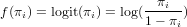
Exercise 12.12 What is the logistic transformed value for an observation of 0, and
of 1?
A simple logistic model can be formed by regressing gender as a function of weight, in the student data set:
Exercise 12.13 Why are the observations not shown in the first plot?
Look at the predicted values for each of the Weight values:
and consider the predicted values from the glm as probabilities of being one (i.e., having gender "male").
Exercise 12.14 [HAND IN] Above which weight value would you predict the
gender of a person with unknown gender as being male?