Contents

1 Linear Regression

in this exercises the basics of linear regression are repeated. we use a dataset stored in R, it needs some preparation.

Exercise 1 Describe the data: meaning of the values, temporal resolution and extent. 

Exercise 2 Plot the data. 

Exercise 3 Use linear regression to fit a line to the data, according to the Model

Exercise 4 Pick a month (e.g. January 1970), what is the mean estimate of the monthly average of CO2 value in this month? 

Exercise 5 According to the fitted model, what is the 95% confidence interval for a single prediction of the monthly average of CO2 in this month? Is the measured value within this confidence interval? 

Exercise 6 [ HAND IN]Is the linear regression line a good model for the data? How could it be improved?

2 Generating random walk data

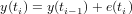
Random walk is generated by the process

Exercise 7 Does a RW process in general increase, decrease, or does it not have a dominant direction? 

Exercise 8 [ HAND IN]Explain why a RW processs has a variance that increases with its length

3 Time series analysis of meteo data

3.1 Exploratory data analysis

The meteo data set is a time series with 1-minute data, collected during a field exercise in the Haute Provence (France), in a small village called Hauteville, near Serres.

What follows is a short description of the variables.

ID

ID of this data logger

year

year

julian.day

day number starting on Jan 1st

time

time, not decimal but as hhmm

T.outside

outside temperature in degrees Celcius

pressure

1000 - pressure, mbar

humidity

humidity, as percentage

X

unknown

windspeed

wind speed

std.dev.

variability of wind speed

Wind.dir

wind direction, in degrees

std.dev..1

variability of wind direction (useless)

TippingBucket

tipping bucket: rain fall in mm/min

date

ISO time

Look at the summary of the meteo data, and plot temperature

3.2 Fitting a periodic component

We will now fit a periodic component to this data, using a non-linear fit.

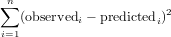
We used the function nlm that will minimize the function in its first argument (f), using the initial guess of the parameter vector in its second argument. The function f computes the sum of squared residuals:

We will now plot observations and fitted model together:

Exercise 10 What is the interpretation of the fitted parameters? (if you need to guess, modify them and replot) 

We can now also plot the residual from this fitted model:

3.3 Fitting AR model to the residuals

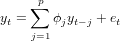
The AR(p) model is defined as

Now try to model the residual process as an AR(5) process, and look at the partial correlations.

(Note that this generates 2 plots)

Exercise 11 Does the an process exhibit temporal correlation for lags larger than 0? 

Exercise 12 Does the residuals(an.ar5) process still exhibit temporal correlation for lags larger than 0? 

Exercise 13 What is the class of the object returned by arima? 

Let us see what we can do with such an object.

Exercise 14 Try to explain what you see in the first two plots obtained 

3.4 Model selection with AIC

Exercise 15 Which model has the smallest AIC? 

Exercise 16 HAND IN: Do a similar analysis for the humidity variable in the meteo data set. (i) Fit a periodic trend; give the trend equation; (ii) Plot the humidity data and the fitted model; (iii) detrend the humidity data to obtain residuals and report for which value of n in an AR(n) model of the model anomalies (residuals) has the lowest AIC. (iv) Up to which lag does the residual humidity process exhibit temporal correlation?  

3.5 Prediction with an AR model

Let us now work with the AR(6) model for the temperature, ignoring the periodic (diurnal) component. Make sure you have "plot recording" on (activate the plot window to get this option).

Exercise 17 Where does, for long-term forecasts, converge the predicted value to? Explain why? 

Now compare this with prediction using an AR(6) model for the residual with respect to the daily cycle:

Exercise 18 [ HAND IN]Where does now, for long-term forecasts, converge the predicted value to? Explain the difference to the upper model.

Exercise 19 [ HAND IN]Fit a periodic trend and AR(3) model to the humidity. Plot predictions for one week.

4 One-dimensional search with golden section

The function optimize (or, for that sake, optimise) optimizes a one-dimensional function. Let us try to fit the phase of a sin function.

The optimization looks quite good, but approximates.

Exercise 20 What was the default tolerance value used here? 

We can make the tolerance smaller, as in

We can check whether more significant digits were fitted correctly:

Exercise 21 Is this fit better? Did optimize get the full 9 (or more) digits right? 

Function optimize uses a combination of golden section search and another approach.

Exercise 22 HAND IN: What is the other approach used? Search for the explanation of this method (English wikipedia), and briefly describe in your own words how it works. Explain why this method is used as well.  

5 Linear and non-linear least squares

As a preparation, go through the course slides; if you missed the lecture you may want to go through the Gauss-Newton algorithm, e.g. on English wikipedia.

5.1 By hand

First, we will try example by “hand”. Consider the following data set:

and try to find the coefficients b₀, b₁ and b₂ of the linear regression equation

Exercise 23 HAND IN: report the values of the coeffients found; compute the residual sum of squares R; report the steps used to compute R and the value found.  

5.2 Linear: by lm

Fit the same model and check your results, found above:

5.3 Non-linear: using nls

Function nls uses a formula as its first argument, and a data frame as its second argument. In the introduction chapter 11, http://cran.r-project.org/doc/manuals/R-intro.html#Statistical-models-in-R, statistical models expressed as formula are explained. The general explanation here is on linear (and generalized linear) models.

Function nls uses, just like lm, a formula to define a model. It differs from lm formulas in that coefficients need to be named explicitly. In linear models, the coefficients are implicit, e.g. linear regression uses the function lm (linear model), and for instance

fits and summarized the linear regression model

For non-linear models, we need to name coefficients explicitly, as they may in principle appear anywhere. In the example below, the now familiar sinus model is refitted using function nls, which uses Gauss-Newton optimization, and the coefficients are named a, b and c in the formula.

5.4 Initial conditions

Try fit the following two models:

The two fits provide different outcomes.

Exercise 24 What does the third argument to nls contain, and why does it change the outcome? 

Exercise 25 Does one of the models give a better fit? 

The following fit:

gives an error message.

Exercise 26 HAND IN: Compute the Jacobian by hand 

Exercise 27 HAND IN: Explain why the error occured. 

5.5 Iteration

The consecutive steps of the optimization are shown when a trace is requested.

Exercise 28 What is the meaning of the four columns of additional output? 

Exercise 29 Why is more than one step needed? 

In the following case

convergence takes place after a single iteration.

Exercise 30 Why was this predictable? 

Compare the following two fits:

5.6 Confidence intervals

Confidence intervals for the coefficients can be computed (or approximated) by the appropriate methods available in library MASS:

Exercise 31 Which coefficients are, with 95% confidence, different from zero? 

5.7 Prediction

Try

to see how predictions are generated for the data points. Interestingly, the two commands

all do the same. Although surprising, it is documented behaviour; see ?predict.nls. Prediction errors or intervals are much harder to obtain for non-linear models than for linear models.

6 Metropolis and Simulated Annealing

6.1 Fun with Metropolis

The Metropolis algorithm is a simplified version of the Metropolis-Hastings algorithm (search English wikipedia), and provides a search algorithm for finding global optima, and sampling the (posterior) parameter distribution, given the data.

Let P(θ) be the probability that parameter value θ has the right value, given the data.

The metropolis algorithm considers proposal values θ′ for the parameter vector, and accepts if, given the current value θ_i, the ratio

• α is larger than one (meaning θ′ is an improvement), or
• when a random value drawn uniformly between 0 and 1 is smaller than α, meaning that we accept worse parameters quite often if they’re not too much worse.

6.2 An R function for MCMC

Consider the following function, and try to understand what is going on:

Then, insert the function in your working environment by copying and pasting the whole block.

To understand why the ratio is computed like it is here, have a look at , the likelihood function for the normal distribution. Also recall that using exp(a)/exp(b) = exp(a-b) is needed for numerical stability.

Let’s try and see if it works. First recollect the non-linear least squares fit with nls and use that as a starting condition:

We can try to see what happened to the three parameters if we plot them. For this we will make a little dedicated plot function, called plot.Metropolis. It will be automatically called for objects of class Metropolis

Here’s the plot function:

that you should load in the environment. Try it with:

Note that now your own plot.Metropolis has been called, because Metropolis is the class of out.

Exercise 32 HAND IN: which percentage of the proposals was rejected, and how could you decrease this percentage? 

Compare the values found with those obtained with nls e.g. by:

6.3 The effect of sigma

Set the plot recording to “on” (activate the plot window, use the menu). Now you can browse previous plots with PgUp and PgDown, when the plot window is active.

Let’s first try a very small sigma.

Exercise 33 HAND IN: (i) which chain becomes stationary, meaning that it fluctuates sufficiently for a long time over the same area? (ii) which of the chains do not mix well?  

6.4 Computing summary statistics

A useful function for doing something for each row or column is apply. Read it’s help page, and try

Another way of looking into the results is by plotting them; one naive plot is

It should however be reminded that a Metropolis chain contains by construction serial correlation; a plot that reveals that is the line plot

Univarite distribution plots can be obtained by hist and qnorm, e.g..

Exercise 34 HAND IN: does parameter x[1] approximately follow a normal distribution? 

6.5 Initial values and Burn-in

Above, we started a Metropolis chain using fitted values from nls; now we will use arbitrary, much worse values:

The burn-in period is the period that the chain needs to go from the initial values to the region where it becomes stationary.

Exercise 35 HAND IN: for the different values of sigma2, how long does it take before the chain becomes stationary?  

Exercise 36 HAND IN: How do you compute (give the R command) the mean and summary statistics for a chain ignoring the burn-in values? 

6.6 Simulated Annealing

Not surprisingly, numeric optimization is an area with many applications in statistics. An overview of all the optimization methods avaible in R and its contributed packages is found by following the links: R web site ⇒ CRAN ⇒ select a CRAN mirror ⇒ Task Views ⇒ Optimization (and while there, please note there is also a Task View on Spatial issues).

Simulated annealing is available as a method provided by the generic optimization function optim. Read the help page of this function and answer the following question.

Exercise 37 HAND IN: why is simulated annealing not a generic-purpose optimization method 

Suppose we want to find the mean, scale and phase of the temperature data, and are looking for the model that best fits in terms of least absolute deviations. Define the function

Exercise 38 HAND IN: What do the various output elements mean? 

Do the

Exercise 39 HAND IN: explain why the parameters are equal/not equal 

Exercise 40 HAND IN: use simulated annealing to find the least squares solution; give the function used, and compare the resulting parameter values with the least absolute error solution.  

7 Spatial modelling: introductory matter

7.1 Data sets

Besides data that are typed in, or data that are imported through import functions such as read.csv, some data are already available in packages. In package gstat for example, a data set called meuse is available. To copy this data set to the current working data base, use, e.g. for the meuse data

7.1.1 meuse

The meuse data set is a data set collected from the Meuse floodplain. The heavy metals analyzed are copper, cadmium, lead and zinc concentrations, extracted from the topsoil of a part of the Meuse floodplain, the area around Meers and Maasband (Limburg, The Netherlands). The data were collected during fieldwork in 1990 (Rikken and Van Rijn, 1993; Burrough and McDonnell, 1998).

Load library gstat by

and read the documentation for the data set by ?meuse)

7.2 Models: the formula interface; linear regression

Most statisticians (and many earth scientists as well) like to analyse data through models: models reflect the hypotheses we entertain, and from fitting models, analysing model output, and analysising graphs of fitted values and residuals we can learn from the data whether a given hypothesis was reasonable or not.

Many models are variations of regression models. Here, we will illustrate an example of a simple linear regression model involving the heavy metal pollution data in meuse. We will entertain the hypothesis that zinc concentration, present in variable zinc, depends linearly on distance to the river, present in dist. We can express dependency of y on x by a formula, coded as y~x. Formulas can have multiple right-hand sides for multiple linear regression, as y~x1+x2; they also can contain expressions (transformations) of variables, as in log(y)~sqrt(x). See ?formula for a full description of the full functionality.

To calculate a linear regression model for the meuse data:

Do the following yourself:

Besides the variety of plots you now obtain, there are many further custom options you can set that can help analysing these data. When you ask help by ?plot, it does not provide very helpful information. To get help on the plot method that is called when plotting an object of class lm, remember that the function called is plot.lm. Read the help of plot.lm by ?plot.lm . You can customize the plot call, e.g. by

In this call, the name of the second function argument is added because the argument panel is in a very late position. Adding the FALSE as a positional argument, as in

will not work as it comes after the ... argument, which may contain an arbitrary number of arguments that are passed to underlying plot routines. But the following two commands (search for the difference!) both work:

Exercise 41  HAND IN: For this regression model, which of the following assumptions underlying linear regression are violated (if any):

• none
• residuals are heteroscedastic (i.e., their variance is not constant over the range of fitted values)
• residuals are not normally distributed (their distribution is for example non-symmetric)
• residuals are heteroscedastic and not normally distributed

and explain how you can tell that this is the case.  

7.3 Spatial data in R: the sp package

The R package sp provides classes and methods for spatial data; currently it can deal with points, grids, lines and polygons. It further provides interfaces to various GIS functions such as overlay, projection and reading and writing of external GIS formats.

7.3.1 Points

Try:

Here, the crucial argument is the coordinates function: it specifies for the meuse data.frame which variables are spatial coordinates. In effect, it replaces the data.frame meuse which has "just" two columns with coordinates with a structure (of class SpatialPointsDataFrame) that knows which columns are spatial coordinates. As a consequence, spplot knows how to plot the data in map-form. If there is any function or data set for which you want help, e.g. meuse, read the documentation: ?meuse , ?spplot etc.

A shorter form for coordinates is by assigning a formula, as in

The function coordinates without assignment retrieves the matrix with coordinate values.

The plot now obtained shows points, but without reference where on earth they lie. You could e.g. add a reference by showing the coordinate system:

but this tells little about what we see. As another option, you can add geographic reference by e.g. lines of rivers, or administrative boundaries. In our example, we prepared the coordinates of (part of) the river Meuse river boundaries, and will add them as reference:

SpatialRings, Srings and Sring create an sp polygon object from a simple matrix of coordinates; the sp.layout argument contains map elements to be added to an spplot plot.

Note that the points in the plot partly fall in the river; this may be attributed to one or more of the following reasons: (i) the river coordinates are not correct, (ii) the point coordinates are not correct, (iii) points were taken on the river bank when the water was low, whereas the river boundary indicates the high water extent of the river.

7.3.2 Grids

Try:

Here, gridded(meuse.grid) = TRUE promotes the (gridded!) points to a structure which knows that the points are on a regular grid. As a consequence they are drawn with filled rectangular symbols, instead of filled circles. (Try the same sequence of commands without the call to gridded() if you are curious what happens if meuse.grid were left as a set of points).

For explanation on the sp.layout argument, read ?spplot; much of the codes in them (pch, cex, col) are documented in ?par.

Note that spplot plots points on top of the grid, and the grid cells on top of the polygon with the river. (When printing to pdf, transparency options can be used to combine both.)

7.4 Import/export: rgdal

R package rgdal provides several drivers for import/export of spatial data. For vector data (points, lines, polygons) an overview is obtained by

for grid data by

The full set of theoretically available drivers with documentation are given here and here.

Export the data set to KML

and import it in google earth.

8 Geostatistics

These practical exercises cover the use of geostatistical applications in environmental research. They give an introduction to exploratory data analysis, sample variogram calculation and variogram modelling and several spatial interpolation techniques. Interpolation methods described and applied are inverse distance interpolation, trend surface fitting, thiessen polygons, ordinary (block) kriging, stratified (block) kriging and indicator (block) kriging.

The gstat R package is used for all geostatistical calculations. See:

E.J. Pebesma, 2004. Multivariable geostatistics in S: the gstat package. Computers & Geosciences 30: 683-691 .

8.1 Exploratory data analysis

Identify the five largest zinc concentrations by clicking them on the plot:

Exercise 42  Which points have the largest zinc concentration:

• 44 51 54 55 82
• 49 53 54 55 82
• 46 53 54 55 82
• 53 54 55 59 82

8.2 Simple interpolation algorithms

8.2.1 Trend surface analysis

Trend surface interpolation is multiple linear regression with polynomials of coordinates as independent, predictor variables. Although we could use lm to fit these models and predict them, it would require scaling of coordinates prior to prediction in most cases because higher powers of large coordinate values result in large numerical errors. The krige function in library gstat scales coordinates and computes trend surface up to degree 3, using scaled coordinates.

Function surf.ls from library spatial (described in the MASS book) fits trends up to order 6 with scaled coordinates.

As you can see, ?krige does not provide help on argument degree. However, tells that any remaining arguments (...) are passed to function gstat, so look for argument degree on ?gstat.

Exercise 43  HAND IN: The danger of extreme extrapolation values is likely to occur

• for low trend orders
• for high trend orders
• for none of these models

Briefly explain why this is the case.  

Local trends, i.e. trends in a local neighbourhood may also be fitted:

8.2.2 Inverse distance interpolation

Inverse distance interpolation calculates a weighted average of points in the (by default global) neighbourhood, using weights inverse proportional to the distance of data locations to the prediction location raised to the power p. This power is by default 2:

The argument set is a list because other parameters can be passed to gstat using this list as well.

Exercise 44  HAND IN: With a larger inverse distance power (idp), the weight of the nearest data point

• becomes larger
• becomes smaller
• does not change

explain in words why this is the case.  

8.2.3 Thiessen polygons

Thiessen polygons can be constructed (as vector objects) using the functions in library tripack. Interpolation on a regular grid is simply obtained by using e.g. inverse distance interpolation and a neighbourhood size of one (nmax = 1). Combining the two:

8.3 Spatial prediction with multiple linear regression

In the data set meuse we have a large number of variables present that can be used to form predictive regression models for either of the heavy metal variables. If we want to use such a regression model for spatial prediction, we need the variables as a full spatial coverage, e.g. in the form of a regular grid covering the study area, as well. Only few variables are available for this in meuse.grid:

Now try:

Exercise 45  Why are prediction standard errors on the log-scale largest for small and large distance to the river?

• Because variability is smallest for intermediate distance to river
• because the uncertainty in the regression slope is most prevalent when the regressor distance takes extreme values
• because we have too few degrees of freedom for regression (i.e., too few observations) overall
• because we have too little data close to the river and far away from the river

We can use the prediction errors provided by lm to calculate regression prediction intervals:

Next, we can make maps of the 95% prediction intervals:

Note that all these prediction intervals refer to prediction of single observations; confidence intervals for mean values (i.e., the regression line alone) are obtained by specifying interval = "confidence".

Exercise 46 Compared to prediction intervals, the intervals obtained by interval = "confidence" are

• wider
• narrower
• of approximately equal width

Another regression model is obtained by relating zinc to flood frequency, try

Exercise 47 Why is a box-and whisker plot drawn for this plot, and not a scatter plot?

• ffreq is a categorical variable with numeric levels
• ffreq has only three values, 1, 2 and 3
• flood frequency is allways expressed by boxes

Exercise 48 What do the boxes in a box-and whisker plot refer to?

• the mean plus and minus one standard deviation of the group
• the 95% confidence interval for the mean
• the inter-quartile range (from 25-th to 75-th percentiles)

Exercise 49 What is needed for flood frequency to use it for mapping zinc?

• it needs to be the number of times a grid cell floods
• it needs to be known at each prediction location (i.e., grid cells in meuse.grid
• it needs to be independent of distance to the river

Try the model in prediction mode:

Exercise 50  HAND IN: Why is the pattern obtained not smooth?  

8.4 Spatial correlation: the h-scatterplot

Before we jump into h-scatterplots of spatial data, let us first (re-)consider lagged scatterplots for temporal data.

Exercise 51 HAND IN: create the lagged scatterplots for the T.outside variable in the meteo data set, for lag 1 und 10. Compute and report the corresponding correlations.  

Read the help for function hscat in package gstat.

We will use this function to compute h-scatterplots. An h-scatterplot plots data pairs z(x_i),z(x_j) for selected pairs that have |x_i -x_j| fall within a given interval. The intervals are given by the third argument, (breaks).

Exercise 52 Why is there not a distance interval 0 - 30 in the plot?  

Exercise 53 HAND IN: how many point pairs can you form from 155 observations? 

Exercise 54 HAND IN: The correlation steadily drops with larger distance. Why? 

Exercise 55 How would you interpret the negative correlation for the largest lag? 

8.5 Spatial correlation: the variogram cloud

As you could see, above the variogram cloud was used to get h-scatterplots. The variogram cloud is basically the plot (or collection of plotted points) of

Plot a variogram cloud for the log-zinc data:

Exercise 56 Why are both distance and semivariance non-negative? 

Exercise 57 Why is there so much scatter in this plot? 

Exercise 58 How many points does the variogram cloud contain if the separation distance is not limited? 

Identify a couple of points in the cloud, and plot the pairs in a map by repeating the following commands a couple of times. The following command lets you select point pairs by drawing polygons around them. Please note the use of the different keys on the mouse.

Exercise 59 HAND IN: Where are the short-distance-high-variability point pairs, as opposed to the short-distance-small-variability point pairs? 

8.6 Spatial correlation: the variogram

A variogram for the log-zinc data is computed, printed and plotted by

Exercise 60 How is the variogram computed from the variogram cloud?

• semivariance is averaged for each distance
• distance is averaged for each semivariance
• distance is averaged for each semivariance class
• semivariance and distance are averaged for each distance class
• semivariance and distance are averaged for each semivariance class

8.7 Sample variogram and variogram model

To detect, or model spatial correlation, we average the variogram cloud values over distance intervals (bins):

For the maximum distance (cutoff) and bin width, sensible defaults are chosen as one-third the largest area diagonal and 15 bins, but we can modify this when needed by setting cutoff and width:

Exercise 61  What is the problem if we set width to e.g. a value of 5?

• we get too many semivariance estimates
• the semivariance values are too large
• the semivariance values are too small
• the variability of the semivariance values is too large

Exercise 62  HAND IN: What is the problem if we set the cutoff value to e.g. a value of 500 and width to 50?

For kriging, we need a suitable, statistically valid model fitted to the sample variogram. The reason for this is that kriging requires the specification of semivariances for any distance value in the spatial domain we work with. Simply connecting sample variogram points, as in

will not result in a valid model. Instead, we will fit a valid parametric model. Some of the valid parametric models are shown by e.g.

These models may be combined, and the most commonly used are Exponential or Spherical models combined by a Nugget model.

We will try a spherical model:

Exercise 63  The range, 1000, relates to

• the semivariance value at distance (nearly) zero
• the semivariance value reached when the variogram stops increasing
• the distance value at which the variogram stops increasing

Exercise 64  The sill, 0.6 + 0.05, relates to

• the semivariance value at distance (nearly) zero
• the semivariance value reached when the variogram stops increasing
• the distance value at which the variogram stops increasing

Exercise 65  The nugget, 0.05, relates to

• the semivariance value at distance (nearly) zero
• the semivariance value reached when the variogram stops increasing
• the distance value at which the variogram stops increasing

The variogram model ("Sph" for spherical) and the three parameters were chosen by eye. We can fit the three parameters also automatically:

but we need to have good "starting" values, e.g. the following will not yield a satisfactory fit:

Exercise 66 HAND IN: Compute the variogram for four different direction ranges (hint: look into argument alpha for function variogram) and plot it in a single plot. Is the zinc process anisotropic? Try to explain what you find in terms of what you know about the process.  

8.8 Simple and ordinary kriging

Ordinary kriging is an interpolation method that uses weighted averages of all, or a defined set of neighbouring, observations. It calculates a weighted average, where weights are chosen such that (i) prediction error variance is minimal, and (ii) predictions are unbiased. The second requirement results in weights that sum to one. Simple kriging assumens the mean (or mean function) to be known; consequently it drops the second requirement and the weights do not have to sum to unity. Kriging assumes the variogram to be known; based on the variogram (or the covariogram, derived from the variogram) it calculates prediction variances.

To load everything you need into your workspace do

8.8.1 Weights

One main advantage of kriging compared to e.g. inverse distance weighting is that it cares about clustering of the points where the values for prediction come from.

Exercise 67 Imagine you want to predict a value by three others. All three points have the same distance from the point to predict, two of them are very close together and the third one is on the opposite side of the point to predict. Which weighting would you choose and why?

• Equal weights on all points.
• Put more weight on the single point than on the two clustered ones.
• Put less weight on the single point than on the two clustered ones.

Download the EZ-Kriging tool to see how weighting is done by kriging (download the .zip file and unzip it, than it can be started by clicking the icon) Use it to answer the following questions.

Exercise 68 HAND IN: Which of the following properties are true/false/the opposite is true for inverse distance interpolation and for kriging, respectively?

• Points closer to the point to predict have more weight.
• Clustered points have more weight.

8.8.2 Influence of Variogram on Prediction

Use EZ-Kriging. Place 7 points, some in a cluster and the others on different distances from the centre singularily.You may keep the values at the points.

The first parameter we look at is the nugget effect. Put the partial sill (c1) to 0 and change the nugget effect (c1).

Exercise 69  What happens to the weights, to the prediction and to the prediction error?  

Can you imagine how the interpolated map looks like? Try pure nugget effect kriging on the log(zinc) data from meuse:

Exercise 70 HAND IN: How are clustered points weighted? How important is the distance to the point to predict? Does pure nugget effect fit data with strong spatial correlation or data where values in different points are uncorrelated?   Exercise 71  What are the predicted values? Explain why this makes sense here!  

Next we explore the range. In EZ-Kriging put c1 back to a medium value (keep the exponential model). Try out different ranges.

Exercise 72  How is the influence of the range on weighting (compare very small, medium and very big range)?  

Try kriging for different ranges on the log(zinc) values.

Repeat for range = 10000 (true range is about 1000).

Exercise 73 HAND IN: Describe the main differences of the kriged map for small/big range and compare the errors?  

Given that lzn.mod a suitable variogram model contains (see above), we can apply ordinary kriging by

For simple kriging, we have to specify in addition the known mean value, passed as argument beta:

Comparing the kriging standard errors:

Exercise 74 HAND IN: Why is the kriging standard error not zero in grid cells that contain data points?

• kriging standard errors are not zero on data points
• the data points do not coincide exactly with grid cell centres
• kriging standard errors do not depend on data locations, they only depend on the variability of measured values

Explain your answer briefly.  

Local kriging is obtained when, instead of all data points, only a subset of points nearest to the prediction location are selected. If we use only the nearest 5 points:

Exercise 75  When we increase the value of nmax, the differences between the local and global kriging will

• become smaller
• become larger
• remain the same

Another, commonly used strategy is to select a kriging neighbourhood based on spatial distance to prediction location. To exagerate the effect of distance-based neighbourhoods, a very small neighbourhood is chosen of 200 m:

Exercise 76  How can the gaps that now occur in the local neighbourhood kriging map be explained? At these prediction locations

• the kriging neighbourhood is empty
• the kriging neighbourhood only contains a single observation
• the kriging neighbourhood contains less than 2 observations

Ordinary and simple kriging behave different in this latter aspect.

Exercise 77 HAND IN: In the areas with gaps in the ordinary kriging map, simple kriging yields

• the simple kriging mean value (5.9)
• a compromise between the mean value (5.9) and the nearest observation
• a compromise between the mean value (5.9) and the nearest two or more observations

Explain why this is the case.  

Some texts advocate to choose search neighbourhood distances equal to the range of the variogram, however there is no theoretical nor a practical justification for this: weights of points beyond the correlation range are usually not zero. Choosing a local neighbourhood may save time and memory when kriging large data sets. In addition, the assumption of a global constant mean is weakened to that of a constant mean within the search neighbourhood. Examine the run time for the following problem: (interpolation of approximately 1000 points with random values).

Randomly select approximately 1000 points:

See how many we obtained:

Create nonsense data from a standard normal distribution; interpolate and plot them:

and compare the run time for global kriging to local kriging with the nearest 20 observations.

Exercise 78  The gain in speed is approximately a factor

• 5
• 10
• 20
• 60

Although not needed here, for exact timings, you can use system.time, but then replace dummy.int = ... with dummy.int <- ... in the expression argument.

8.9 Universal kriging

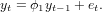
Just like stratified kriging, universal kriging provides a less restrictive model than ordinary kriging. Suppose the model for ordinary kriging is written as

Universal kriging extends the ordinary kriging model by replacing the constant mean value by a non-constant mean function:

The hope is that the predictor functions carry information in them that explains the variability of Z(s) to a considerable extent, in which case the residual e(s) will have lower variance and less spatial correlation compared to the ordinary kriging case. To see that this model extends ordinary kriging, take p = 0 and note that for that case β₀ = m. Another simplification is that if e(s) is spatially independent, the universal kriging model reduces to a multiple linear regression model. One problem with universal kriging is that we need the variogram of the residuals, without having measured the residuals.

As we’ve seen before, we can predict the zinc concentrations fairly well from the sqrt-transformed values of distance to river:

To compare the variograms from raw (but log-transformed) data and regression residuals, look at the conditioning plot obtained by

Exercise 79  How is the residual standard error from the regression model above (lzn.lm) related to the variogram of the residuals:

• it is half the mean semivariance of the raw data and that of the residuals
• the square of the residual standard error (the residual variance) equals the sill of the residual variogram
• it equals the range of the residual variogram
• it equals the sill of the residual variogram
• it equals the nugget of the residual variogram
• the residual variance (approximately) equals the nugget of the variogram

Exercise 80  HAND IN: Why is the sill of the residual variogram much lower than the sill of the variogram for the raw data?  

When a regression model formula is passed to variogram, the variogram of the residuals is calculated. When a model formula is passed to krige, universal kriging is used.

Now model the residual variogram with an exponential model, say zn.res.m, and apply universal kriging. Compare the maps with predictions from universal kriging and ordinary kriging in a single plot (with a single scale), using spplot.

Exercise 81  Where are the differences most prevalent:

• In areas with values for dist close to 0 and 1
• In areas with few data points
• In areas where both (a) and (b) are valid

Exercise 82  Why are the differences happening exactly there?

• on locations far from measurements, interpolation relies heavily on the estimated trend value; where dist is close to 0 or 1, the trend value is most different from the value m used in ordinary kriging
• on locations far from measurements we are most uncertain about the true values
• on locations where dist is close to 0 or 1, it was hard to collect data, because these locations were hard to reach.

Now print the maps with prediction errors for ordinary kriging and universal kriging with a single scale. See if you can answer the previous two questions in the light of the differences between prediction errors.

8.10 Regression coefficients

Gstat can be (mis-)used to obtain estimates under the full linear model with spatial correlation. Try the following commands:

Exercise 83 What is calculated here (two correct answers)?

• The universal kriging trend for log(zinc) at the points in newdat .
• The universal kriging prediction at these points.
• The universal kriging prediction at these points using only sqrt(dist) for prediction.
• The value for the parameter of the kriging trend.

  Exercise 84 Do the values calculated above depend on the location of the point, why? Do they depend on the variogram (lzn.mod), why? 

Compare the above obtained regression coefficients with those obtained from function lm

Exercise 85 HAND IN: explain why both sets of fitted coefficients, and their standard errors, are different 

8.11 Block kriging

We will try block kriging settings under the universal kriging model. Note that the grid cell size of meuse.grid is 40:

meaning that blocks of size 400 are largely overlapping.

Exercise 86 HAND IN: Describe what happens if we change from point prediction to block prediction of size 40, in terms of predictions and in terms of prediction standard errors? 

Exercise 87 HAND IN: Describe what happens if we change from block prediction for blocks of size 40 m to block prediction for blocks of size 400 m, in terms of predictions and in terms of prediction standard errors? 

You can select a particular point in an object of class SpatialPixelsDataFrame, based on coordinates, e.g. by

Exercise 88 What is the average (predicted by kriging) value of log(zinc) in the 400 x 400 block with center x = 179020, y = 330620? What is the kriging variance there? Why is the kriging variance lower than in the block with centre in x = 180500, y = 332020?  

Exercise 89 HAND IN: give the four corner points of the block mentioned in the previous exercise 

Compare the lowest standard error found with the standard error of the mean in a simple linear regression (with a mean only):

Exercise 90 HAND IN: why is the block mean value for the mean of the complete area different from the sample mean value of the log(zinc) observations? 

8.12 Cokriging

Exercise 91  Which of the parameters (nugget, partial sill, range, model type) were fitted in the above call to fit.lmc?  

Do a cokriging:

Exercise 92 HAND IN: explain in language (without equations) what the variables in the resulting object represent, and how they were computed 

Exercise 93 HAND IN: explain why all the prediction error covariances are positive 

We want to compute an index of toxicity of the soil, where the different heavy metals are weighted according to their toxicity. The index is computed as

Exercise 94 HAND IN: give the R commands to compute this index and to show a map of it. Also give the commands to compute the standard error of the index, taking the error covariances into account.  

Exercise 95 HAND IN: how much does the standard error of this toxicity index change as a result of taking the covariances into account, as opposed to ignoring them?  

8.13 Cokriging: the undersampled case

Take a subsample of zinc, called meuse1:

create a multivariate object with subsample of zinc, and full sample of lead:

cokrige:

compare the differences of kriging the 50 observations of zinc with the cokriging of from 50 zinc and 155 lead observations:

Exercise 96 HAND IN: why are the standard errors smaller in the cokriging case? 

8.14 Kriging errors and confidence intervals

Given that we are not certain about zinc levels at locations where we did not measure it (i.e., interpolated grid cells) we can classify them according to their approximate confidence intervals, formed by using mean and standard error (here: on the log scale).

Exercise 97 HAND IN: for which fraction of the total area is zinc concentration lower than 500 ppm, with 95% confidence? Give the number of grid cells for which this is the case, and describe where in the area they are situated.  

For a single threshold, we can vary the confidence level by specifying alpha:

Exercise 98 HAND IN: which of these four maps has the highest confidence level, and what is this level? Why are there gray areas on map ci050 at all? 

Consider the object zn, created under the section of block kriging.

Exercise 99 HAND IN: compare the fraction classified as lower and higher between ok_point and uk_point, and try to explain the difference 

Exercise 100 HAND IN: compare the fraction classified as lower and higher between uk_point, uk_block40 and uk_block400, and try to explain the difference 

8.15 Conditional simulation

Exercise 101 HAND IN: create a sample of 12 conditional simulations, for log-zinc concentrations, using the krige command, and plot them. Make sure you set nmax to a limited value (e.g. 40). Compare the outcomes, and describe in which respects they differ, and in which respect they are similar.  

8.16 Cross validation

For cross validating kriging resulst, the functions krige.cv (univariate) and gstat.cv (multivariate) can be used.

Exercise 102 HAND IN: perform cross validation for three diffferent (e.g. previously evaluated) kriging types/models using one of these two functions. Compare the resulst at least based on (i) mean error, (ii) mean square error, (iii) mean and variance of the z-score, and (iv) map of residuals (use function bubble for the residual variable). Compare on the results, and compare them to the ideal value for the evaluated statistics/graph.  

9 Diffusion and partial differential equations

Consider the following function, that solves a 1-D diffusion equation, using backward differencing, and plots the result. Do the following exercises after you studied the material (slides/podcast) on differential equations. The following

If you want to safe graphs in an efficient way (for once, a bitmap), you could use e.g.

Try the following:

Exercise 103  [HAND IN:] Which process is described by this model (hint: lecture)? What does it do?  

Use the following commands to have a closer look

Exercise 104  What is the meaning of the different parameters (dt, dx, n.end, x.end)? Try them! What can be seen on these plots compared to the initial ones?  

Exercise 105 [HAND IN:] What happens if dt is close but below 0.5, at 0.5, above 0.5? Find plots to show it, describe and explain with help of them.  

Exercise 106  How could the problem be solved (hint: change other parameters)?  

Try

Exercise 107 What is the total (sum) of out, after the last time step, for the last two commands? What has happened to the material released? 

Exercise 108  What does the Dirichlet boundary condition mean for the values?  

Exercise 109 [HAND IN:] In case of dirichlet =TRUE: What happens to the released material until the last time step (calculate the total sum of out)? What has happened at earlier time steps (calculate a few numbers to describe it)?  

Exercise 110 [HAND IN:] In case of dirichlet =FALSE: What are the conditions at the boundaries? What happens to the released material (total sum of out)?  

Use the following command

Change one parameter at each step, the others shall stay in the original state.

Exercise 111  What is the concentration (out) at the points 20 steps from the release point after 1000 time steps (n.end = 1000)? Why? How does it change when release is half ? Why? How does it change when dt is half? Why? How does it change when dirichlet = TRUE? Why?  

Exercise 112 [HAND IN:] Hand in a short description of your plan for the assignment: which data will you analyze, what kind of hypothesis do you want to look at, which type of analysis methods will you use