Contents

1 Introduction to R

1.1 S, S-Plus and R

S is a language for data analysis and statistical computing. It has currently two implementations: one commercial, called S-Plus, and one free, open source implementation called R. Both have advantages and disadvantages.

S-Plus has the (initial) advantage that you can work with much of the functionality without having to know the S language: it has a large, extensively developed graphical user interface. R works by typing commands (although the R packages Rcmdr and JGR do provide graphical user interfaces). Compare typing commands with sending SMS messages: at first it seems clumsy, but when you get to speed it is fun.

Compared to working with a graphical program that requires large amounts of mouse clicks to get something done, working directly with a language has a couple of notable advantages:

• after a few commands, you can exactly (i) see and (ii) replicate what you did, and send the list of commands to someone else to replicate your analysis;
• when you have a large number of analyses that take much time, you can easily perform them as batches, possibly on a remote computer or on a cluster of computers;
• when you tend to repeat a set of commands often, you can very easily turn them into an S function, which then extends the language, is available forever, and can be redistributed. In the world of R, users soon become developers–vice versa, most developers are users in the first place.

Of course the disadvantage (as you may consider it right now) is that you need to learn a few new ideas.

Although S-Plus and R are both full-grown statistical computing engines, throughout this course we use R for the following reasons: (i) it is free (S-Plus may cost in the order of 10,000 USD), (ii) development and availability of novel statistical computation methods is much faster in R.

Recommended text books that deal with both R and S-Plus are e.g.:

1. W. Venables, B. Ripley: Modern applied statistics with S; Springer (emphasizes on statistical analysis)
2. W. Venables, B. Ripley: S Programming; Springer (emphasizes on programming)
3. J. Chambers: Programming with Data; Springer (fundamental; written by one of the designers of S)

Further good books on R are:

1. P. Dalgaard, Introductory Statistics with R; Springer

1.2 Downloading and installing R

To download R on a MS-Windows computer, do the following:

1. point your web browser to http://www.r-project.org
2. click on the link to CRAN (abbreviation of the Comprehensive R Archive Network)
3. choose a nearby mirror
4. click on the MS-Windows version of R
5. open the self-extracting executable, and follow the instructions

Instructions for installing R on a Macintosh computer are also found on CRAN. For installing R on a linux machine, you can download the R source code from CRAN, and follow the compilation and installation instructions; usually this involves the commands ./configure; make; make install. There may be binary distributions for linux distributions such as RedHat FC, or Debian unstable.

1.3 Starting R; saving or resoring an R session

You can start an R session on a MS-Windows machine by double-clicking the R icon, or through the Start menu (Note that this is not true in the ifgi CIP pools: here you have to find the executable in the right direction on the C: drive). When you start R, you’ll see the R console with the > prompt, on which you can give commands.

Another way of starting R is when you have a data file associated with R (meaning it ends on .RData). If you click on this file, R is started and reads at start-up the data in this file.

Try this using the meteo.RData file. Next, try the following commands:

(Note that you can copy and paste the commands including the > to the R prompt, only if you use "paste as commands")

You can see that your R workspace now has two objects in it. You can find out which class these objects belong by

If you want to remove an object, use

If you want so safe a (modified) work space to a file, you use

2 Generating random walk data

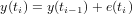
Random walk is generated by the process

Exercise 2.1  Does a RW process in general increase, decrease, or does it not have a dominant direction? 

Exercise 2.2  Explain why a RW processs has a variance that increases with its length 

3 Time series analysis of meteo data

3.1 Exploratory data analysis

The meteo data set is a time series with 1-minute data, collected during a field exercise in the Haute Provence (France), in a small village called Hauteville, near Serres.

What follows is a short description of the variables.

ID

ID of this data logger

year

year

julian.day

day number starting on Jan 1st

time

time, not decimal but as hhmm

T.outside

outside temperature in degrees Celcius

pressure

1000 - pressure, mbar

humidity

humidity, as percentage

X

unknown

windspeed

wind speed

std.dev.

variability of wind speed

Wind.dir

wind direction, in degrees

std.dev..1

variability of wind direction (useless)

TippingBucket

tipping bucket: rain fall in mm/min

date

ISO time

Look at the summary of the meteo data, and plot temperature

3.2 Fitting a periodic component

We will now fit a periodic component to this data, using a non-linear fit.

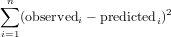
We used the function nlm that will minimize the function in its first argument (f), using the initial guess of the parameter vector in its second argument. The function f computes the sum of squared residuals:

We will now plot observations and fitted model together:

Exercise 3.4  What is the interpretation of the fitted parameters? (if you need to guess, modify them and replot) 

We can now also plot the residual from this fitted model:

3.3 Fitting AR model to the residuals

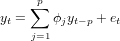
The AR(p) model is defined as

Now try to model the residual process as an AR(5) process, and look at the partial correlations.

(Note that this generates 2 plots)

Exercise 3.5  Does the an process exhibit temporal correlation for lags larger than 0? 

Exercise 3.6  Does the residuals(an.ar5) process still exhibit temporal correlation for lags larger than 0? 

Exercise 3.7  What is the class of the object returned by arima? 

Let us see what we can do with such an object.

Exercise 3.8  Try to explain what you see in the first two plots obtained 

3.4 Model selection with AIC

Exercise 3.9  Which model has the smallest AIC? 

3.5 Prediction with an AR model

Let us now work with the AR(6) model for the temperature, ignoring the periodic (diurnal) component. Make sure you have "plot recording" on (activate the plot window to get this option).

Exercise 3.10  Where does, for long-term forecasts, converge the predicted value to? 

Now compare this with prediction using an AR(6) model for the residual with respect to the daily cycle:

Exercise 3.11  Where does now, for long-term forecasts, converge the predicted value to? 

4 One-dimensional search with golden section

The function optimize (or, for that sake, optimise) optimizes a one-dimensional function. It uses a combination of golden section search and another approach.

Exercise 4.12  Which other approach? 

Let us fit the phase of a sin function.

The optimization looks quite good, but approximates.

Exercise 4.13  What was the tolerance value used here? 

We can make the tolerance smaller, as in

Exercise 4.14  Is this fit acceptable? 

We can check whether more significant digits were fitted correctly:

Exercise 4.15  did optimize get the full 9 (or more) digits right? 

5 Non-linear least squares with nls

As a preparation, go through the course slides; if you missed the lecture you may want to go through the wikipedia pages for golden section search and the Gauss-Newton algorithm.

Function nls uses a formula as its first argument, and a data frame as its second argument. In the introduction chapter 11, http://cran.r-project.org/doc/manuals/R-intro.html#Statistical-models-in-R, statistical models expressed as formula are explained. The general explanation here is on linear (and generalized linear) models.

Formulas form perhaps the most powerful feature of the S language. They are used everywhere when specifying some sort of statistical dependency. The general form, for dependent variable y and independent variable x, is

Today however, we use formulas for non-linear models. The difference is that in linear models the coefficients are implicit, e.g. linear regression uses the function lm (linear model), and for instance

fits and summarized the linear regression model

For non-linear models, we need to name coefficients explicit. In the example below, the now familiar sinus model is refitted using function nls, which uses Gauss-Newton optimization, and the coefficients are named a, b and c in the formula.

5.1 Initial conditions

Try fit the following two models:

The two fits provide different outcomes.

Exercise 5.16  What does the third argument to nls contain? 

Exercise 5.17  Which of the fitted models is better? 

Exercise 5.18  How can you explain the differences? 

The following fit:

gives an error message.

Exercise 5.19  Explain why the error occured. 

Exercise 5.20  Which element(s) of the Jacobian may have been difficult to compute in the first iteration? 

5.2 Iteration

The consecutive steps of the optimization are shown when a trace is requested.

Exercise 5.21  What is the meaning of the four columns of additional output? 

Exercise 5.22  Why is more than one step needed? 

In the following case

convergence takes place after a single iteration.

Exercise 5.23  Why was this predictable? 

Compare the following two fits:

5.3 Confidence intervals

Confidence intervals can be computed (or approximated) by the appropriate methods available in library MASS:

Exercise 5.24  Which coefficients are, with 95% confidence, different from zero? 

5.4 Prediction

Try

to see how predictions are generated for the data points. Interestingly, the two commands

all do the same. But that is documented behaviour; see ?predict.nls. Prediction errors or intervals are much harder to do for non-linear models than for linear models.

6 Fun with Metropolis

The Metropolis algorithm is a simplified version of the Metropolis-Hastings algorithm (search English wikipedia), and provides a search algorithm for finding global optima, and sampling the (posterior) parameter distribution, given the data.

Let P(θ) be the probability that parameter value θ has the right value, given the data.

The metropolis algorithm considers proposal values θ′ for the parameter vector, and accepts if, given the current value θ_i, the ratio

• α is larger than one (meaning θ′ is an improvement), or
• when a random value drawn uniformly between 0 and 1 is smaller than α, meaning that we accept worse parameters quite often if they’re not too much worse.

6.1 An R function for MCMC

Consider the following function, and try to understand what is going on:

Then, insert the function in your working environment by copying and pasting the whole block.

Let’s try and see if it works:

We can try to see what happened to the three parameters if we plot them. For this we will make a little dedicated plot function, called plot.Metropolis. It will be automatically called for objects of class Metropolis

Here’s the plot function:

that you should load in the environment. Try it with:

Note that now your own plot.Metropolis has been called, because Metropolis is the class of out.

Exercise 6.25  Recall the fitted values for the three parameters, found by Gauss-Newton fitting; write them down and compare them with the values you find now. What is different? 

Exercise 6.26  Are the simulated values on average right? 

6.2 The effect of sigma

Set the plot recording on (activate the plot window, use the menu). Now you can browse previous plots with PgUp and PgDown, when the plot window is active.

Let’s first try a very small sigma.

Exercise 6.27  Does the chain for the three parameters become stationary, meaning that it fluctuates for a long time over the same area?  Exercise 6.28  What does the acceptance rate mean? 

Try the same for a larger value for sigma:

Exercise 6.29  Does the chain for the three parameters become stationary, meaning that it fluctuates for a long time over the same area?  Exercise 6.30  How did the acceptance rate change? 

Exercise 6.31  Does the chain for the three parameters become stationary, meaning that it fluctuates for a long time over the same area?  Exercise 6.32  How did the acceptance rate change? 

Exercise 6.33  Does the chain for the three parameters become stationary, meaning that it fluctuates for a long time over the same area?  Exercise 6.34  How did the acceptance rate change? 

Exercise 6.35  Does the chain for the three parameters become stationary, meaning that it fluctuates for a long time over the same area?  Exercise 6.36  How did the acceptance rate change? 

Exercise 6.37  Does the chain for the three parameters become stationary, meaning that it fluctuates for a long time over the same area?  Exercise 6.38  How did the acceptance rate change? 

6.3 Fixing the phase

It might be the case that the phase fitting disturbs the process – after all, any value of x[3]+24 is another equally well fitted value. Suppose we fix it to 1.5:

Exercise 6.39  Is the result now more stationary than without the fixed phase? 

6.4 Computing summary statistics

A useful function for doing something for each row or column is apply. Read it’s help page, and try

Exercise 6.40  How do you interpret the result? 

6.5 Initial values and Burn-in

Up to now, we have tried zero initial values, as in

The burn-in period is the period that the chain needs to go from the initial values to the region where it becomes stationary.

Exercise 6.41  How long (how many steps) is the burn-in period for the above example? 

Exercise 6.42  How do you compute the mean and summary statistics for a chain without the burn-in values? 

Exercise 6.43  How does the burn-in period change when sigma decreases? 

7 Spatial modelling: introductory matter

7.1 Data sets

Besides data that are typed in, or data that are imported through import functions such as read.csv, some data are already available in packages. In package gstat for example, a data set called meuse is available. To copy this data set to the current working data base, use, e.g. for the meuse data

7.1.1 meuse

The meuse data set is a data set collected from the Meuse floodplain. The heavy metals analyzed are copper, cadmium, lead and zinc concentrations, extracted from the topsoil of a part of the Meuse floodplain, the area around Meers and Maasband (Limburg, The Netherlands). The data were collected during fieldwork in 1990 (Rikken and Van Rijn, 1993; Burrough and McDonnell, 1998).

Try and read:

(if this does not work, simply use question mark followed by meuse, as in ?meuse)

7.2 Models: the formula interface; linear regression

Most statisticians (and many earth scientists as well) like to analyse data through models: models reflect the hypotheses we entertain, and from fitting models, analysing model output, and analysising graphs of fitted values and residuals we can learn from the data whether a given hypothesis was reasonable or not.

Models are often variations of regression models. Here, we will illustrate an example of a simple linear regression model involving the heavy metal pollution data in meuse. We will entertain the hypothesis that zinc concentration, present in variable zinc, depends linearly on distance to the river, present in dist. We can express dependency of y on x by a formula, coded as y~x. Formulas can have multiple right-hand sides for multiple linear regression, as y~x1+x2; they also can contain expressions (transformations) of variables, as in log(y)~sqrt(x). See ?formula for a full description of the full functionality.

To calculate a linear regression model for the meuse data:

Do the following yourself:

Besides the variety of plots you now obtain, there are many further custom options you can set that can help analysing these data. When you ask help by ?plot, it does not provide very helpful information. To get help on the plot method that is called when plotting an object of class lm, remember that the function called is plot.lm. Read the help of plot.lm by ?plot.lm or:

and customize the plot call, e.g. by

In this call, the name of the second function argument is added because the argument panel is on position four. An alternative form is:

which passes panel.smooth as argument number 4, without giving its name. The first form is strongly recommended because it is less prone to error, and more readable. Furthermore, argument names are less likely to change over time (living software does change!) than argument order.

Exercise 7.44   Which of the following assumptions underlying linear regression are violated (if any):

• none
• residuals are heteroscedastic (i.e., their variance is not constant over the range of fitted values)
• residuals are not normally distributed (their distribution is for example non-symmetric)
• residuals are heteroscedastic and not normally distributed

7.3 Spatial data in R: the sp package

The R package sp provides classes and methods for spatial data; currently it can deal with points, grids, lines and polygons. It further provides interfaces to various GIS functions such as overlay, projection and reading and writing of external GIS formats.

7.3.1 Points

Try:

Here, the crucial argument is the coordinates function: it specifies for the meuse data.frame which variables are spatial coordinates. In effect, it replaces the data.frame meuse which has "just" two columns with coordinates with a structure (of class SpatialPointsDataFrame) that knows which columns are spatial coordinates. As a consequence, spplot knows how to plot the data in map-form. If there is any function or data set for which you want help, e.g. meuse, read the documentation: ?meuse , ?spplot etc.

A shorter form for coordinates is by assigning a formula, as in

The function coordinates without assignment retrieves the matrix with coordinate values.

The plot now obtained shows points, but without reference where on earth they lie. You could e.g. add a reference by showing the coordinate system:

but this tells little about what we see. As another option, you can add geographic reference by e.g. lines of rivers, or administrative boundaries. In our example, we prepared the coordinates of (part of) the river Meuse river boundaries, and will add them as reference:

SpatialRings, Srings and Sring create an sp polygon object from a simple matrix of coordinates; the sp.layout argument contains map elements to be added to an spplot plot.

Note that the points in the plot partly fall in the river; this may be attributed to one or more of the following reasons: (i) the river coordinates are not correct, (ii) the point coordinates are not correct, (iii) points were taken on the river bank when the water was low, whereas the river boundary indicates the high water extent of the river.

7.3.2 Grids

Try:

Here, gridded(meuse.grid) = TRUE promotes the (gridded!) points to a structure which knows that the points are on a regular grid. As a consequence they are drawn with filled rectangular symbols, instead of filled circles. (Try the same sequence of commands without the call to gridded() if you are curious what happens if meuse.grid were left as a set of points).

For explanation on the sp.layout argument, read ?spplot; much of the codes in them (pch, cex, col) are documented in ?par.

Note that spplot plots points on top of the grid, and the grid cells on top of the polygon with the river. (When printing to pdf, transparency options can be used to combine both.)

8 Geostatistics

These practical exercises cover the use of geostatistical applications in environmental research. They give an introduction to exploratory data analysis, sample variogram calculation and variogram modelling and several spatial interpolation techniques. Interpolation methods described and applied are inverse distance interpolation, trend surface fitting, thiessen polygons, ordinary (block) kriging, stratified (block) kriging and indicator (block) kriging.

The gstat R package is used for all geostatistical calculations. See:

E.J. Pebesma, 2004. Multivariable geostatistics in S: the gstat package. Computers & Geosciences 30: 683-691 .

8.1 Exploratory data analysis

Identify the five largest zinc concentrations by clicking them on the plot:

Exercise 8.45   Which points have the largest zinc concentration:

• 44 51 54 55 82
• 49 53 54 55 82
• 46 53 54 55 82
• 53 54 55 59 82

8.2 Simple interpolation algorithms

8.2.1 Trend surface analysis

Trend surface interpolation is multiple linear regression with polynomials of coordinates as independent, predictor variables. Although we could use lm to fit these models and predict them, it would require scaling of coordinates prior to prediction in most cases because higher powers of large coordinate values result in large numerical errors. The krige function in library gstat scales coordinates and allows trend surface up to degree 3.

Function surf.ls from library spatial (described in the MASS book) fits trends up to order 6 with scaled coordinates.

As you can see, ?krige does not provide help on argument degree. However, tells that any remaining arguments (...) are passed to function gstat, so look for argument degree on ?gstat.

Exercise 8.46   The danger of extreme extrapolation values is likely to occur

• for low trend orders
• for high trend orders
• for none of these models

Local trends, i.e. trends in a local neighbourhood may also be fitted:

8.2.2 Inverse distance interpolation

Inverse distance interpolation calculates a weighted average of points in the (by default global) neighbourhood, using weights inverse proportional to the distance of data locations to the prediction location raised to the power p. This power is by default 2:

The argument set is a list because other parameters can be passed to gstat using this list as well.

Exercise 8.47   With a larger inverse distance power (idp), the weight of the nearest data point

• becomes larger
• becomes smaller
• does not change

8.2.3 Thiessen polygons

Thiessen polygons can be constructed (as vector objects) using the functions in library tripack. Interpolation on a regular grid is simply obtained by using e.g. inverse distance interpolation and a neighbourhood size of one (nmax = 1). Combining the two:

8.3 Spatial prediction with multiple linear regression

In the data set meuse we have a large number of variables present that can be used to form predictive regression models for either of the heavy metal variables. If we want to use such a regression model for spatial prediction, we need the variables as a full spatial coverage, e.g. in the form of a regular grid covering the study area, as well. Only few variables are available for this in meuse.grid:

Now try:

Exercise 8.48   Why are prediction standard errors largest for small and large distance to the river?

• Because variability is smallest for intermediate distance to river
• because the uncertainty in the regression slope is most prevalent when the regressor distance takes extreme values
• because we have too few degrees of freedom for regression (i.e., too few observations) overall
• because we have too little data close to the river and far away from the river

We can use the prediction errors provided by lm to calculate regression prediction intervals:

Next, we can make maps of the 95% prediction intervals:

Note that all these prediction intervals refer to prediction of single observations; confidence intervals for mean values (i.e., the regression line alone) are obtained by specifying interval = "confidence".

Exercise 8.49  Compared to prediction intervals, the intervals obtained by interval = "confidence" are

• wider
• narrower
• of approximately equal width

Another regression model is obtained by relating zinc to flood frequency, try

Exercise 8.50  Why is a box-and whisker plot drawn for this plot, and not a scatter plot?

• ffreq is a categorical variable with numeric levels
• ffreq has only three values, 1, 2 and 3
• flood frequency is allways expressed by boxes

Exercise 8.51  What do the boxes in a box-and whisker plot refer to?

• the mean plus and minus one standard deviation of the group
• the 95% confidence interval for the mean
• the inter-quartile range (from 25-th to 75-th percentiles)

Exercise 8.52  What is needed for flood frequency to use it for mapping zinc?

• it needs to be the number of times a grid cell floods
• it needs to be known at each prediction location (i.e., grid cells in meuse.grid
• it needs to be independent of distance to the river

Try the model in prediction mode:

Exercise 8.53   Why is the pattern obtained not smooth?  

8.4 Spatial correlation: the h-scatterplot

Enter the following R function in your session (don’t feel frustrated if you do not understand what is going on):

We will use this function to compute h-scatterplots. An h-scatterplot plots data pairs z(x_i),z(x_j) for selected pairs that have |x_i -x_j| fall within a given interval. The intervals are given by the third argument, (breaks).

Exercise 8.54  Why is there not a distance interval 0 - 30 in the plot?  

Exercise 8.55   One would expect the correlation to decrease for larger distances. This does not happen. Why?  

Exercise 8.56  The correlation now steadily drops with larger distance. Why? 

Exercise 8.57  The correlation for the largest distance interval is negative. How is this possible? 

8.5 Spatial correlation: the variogram cloud

As you could see, above the variogram cloud was used to get h-scatterplots. The variogram cloud is basically the plot (or collection of plotted points) of

Plot a variogram cloud for the log-zinc data:

Exercise 8.58  Why are there so many points? 

Exercise 8.59  Why are both distance and semivariance non-negative? 

Exercise 8.60  Why is there so much scatter in this plot? 

Exercise 8.61  How many points does the variogram cloud contain if the separation distance is not limited? 

Identify a couple of points in the cloud, and plot the pairs in a map by repeating the following commands a couple of times.

Exercise 8.62  Where are the short-distance-high-variability point pairs, as opposed to the short-distance-small-variability point pairs? 

8.6 Spatial correlation: the variogram

A variogram for the log-zinc data is computed, printed and plotted by

Exercise 8.63  How is the variogram computed from the variogram cloud?

• semivariance is averaged for each distance
• distance is averaged for each semivariance
• distance is averaged for each semivariance class
• semivariance and distance are averaged for each distance class
• semivariance and distance are averaged for each semivariance class

8.7 Sample variogram and variogram model

To detect, or model spatial correlation, we average the variogram cloud values over distance intervals (bins):

For the maximum distance (cutoff) and bin width, sensible defaults are chosen as one-third the largest area diagonal and 15 bins, but we can modify this when needed by setting cutoff and width:

Exercise 8.64   What is the problem if we set width to e.g. a value of 5?

• we get too many semivariance estimates
• the semivariance values are too large
• the semivariance values are too small
• the variability of the semivariance values is too large

Exercise 8.65   What is the problem if we set the cutoff value to e.g. a value of 500 and width to 50?

• we cannot see up to which distance the data are spatially correlated
• the semivariance values are too large
• the semivariance values are too small
• we cannot see if data are spatially correlated

For kriging, we need a suitable, statistically valid model fitted to the sample variogram. The reason for this is that kriging requires the specification of semivariances for any distance value in the spatial domain we work with. Simply connecting sample variogram points, as in

will not result in a valid model. Instead, we will fit a valid parametric model. Some of the valid parametric models are shown by e.g.

These models may be combined, and the most commonly used are Exponential or Spherical models combined by a Nugget model.

We will try a spherical model:

Exercise 8.66   The range, 1000, relates to

• the semivariance value at distance (nearly) zero
• the semivariance value reached when the variogram stops increasing
• the distance value at which the variogram stops increasing

Exercise 8.67   The sill, 0.6 + 0.05, relates to

• the semivariance value at distance (nearly) zero
• the semivariance value reached when the variogram stops increasing
• the distance value at which the variogram stops increasing

Exercise 8.68   The nugget, 0.05, relates to

• the semivariance value at distance (nearly) zero
• the semivariance value reached when the variogram stops increasing
• the distance value at which the variogram stops increasing

The variogram model ("Sph" for spherical) and the three parameters were chosen by eye. We can fit the three parameters also automatically:

but we need to have good "starting" values, e.g. the following will not yield a satisfactory fit:

8.8 Simple and ordinary kriging

Ordinary kriging is an interpolation method that uses weighted averages of all, or a defined set of neighbouring, observations. It calculates a weighted average, where weights are chosen such that (i) prediction error variance is minimal, and (ii) predictions are unbiased. The second requirement results in weights that sum to one. Simple kriging assumens the mean (or mean function) to be known; consequently it drops the second requirement and the weights do not have to sum to unity. Kriging assumes the variogram to be known; based on the variogram (or the covariogram, derived from the variogram) it calculates prediction variances.

Given that lzn.mod a suitable variogram model contains, we can apply ordinary kriging by

For simple kriging, we have to specify in addition the known mean value, passed as argument beta:

Comparing the kriging standard errors:

Exercise 8.69  Why is the kriging standard error not zero on grid cells that contain data points?

• kriging standard errors are not zero on data points
• the data points do not coincide exactly with grid cell centres
• kriging standard errors do not depend on data locations, they only depend on the variability of measured values

Local kriging is obtained when, instead of all data points, only a subset of points nearest to the prediction location are selected. If we use only the nearest 5 points:

Exercise 8.70   When we increase the value of nmax, the differences between the local and global kriging will

• become smaller
• become larger
• remain the same

Another, commonly used strategy is to select a kriging neighbourhood based on spatial distance to prediction location. To exaggerate the effect of distance-based neighbourhoods, a very small neighbourhood is chosen of 200 m:

Exercise 8.71   How can the gaps that now occur in the local neighbourhood kriging map be explained? At these prediction locations

• the kriging neighbourhood is empty
• the kriging neighbourhood only contains a single observation
• the kriging neighbourhood contains less than 2 observations

Ordinary and simple kriging behave different in this latter aspect.

Exercise 8.72   In the areas with gaps in the ordinary kriging map, simple kriging yields

• the simple kriging mean value (5.9)
• a compromise between the mean value (5.9) and the nearest observation
• a compromise between the mean value (5.9) and the nearest two or more observations

Some texts advocate to choose search neighbourhood distances equal to the range of the variogram, however there is no theoretical nor a practical justification for this: weights of points beyond the correlation range are usually not zero. Choosing a local neighbourhood may save time and memory when kriging large data sets. In addition, the assumption of a global constant mean is weakened to that of a constant mean within the search neighbourhood. Examine the run time for the following problem: (interpolation of approximately 1000 points with random values).

Randomly select approximately 1000 points:

See how many we obtained:

Create nonsense data from a standard normal distribution; interpolate and plot them:

and compare the run time for global kriging to local kriging with the nearest 20 observations.

Exercise 8.73   The gain in speed is approximately a factor

• 5
• 10
• 20
• 60

Although not needed here, for exact timings, you can use system.time, but then replace dummy.int = ... with dummy.int <- ... in the expression argument.

8.9 Universal kriging

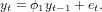
Just like stratified kriging, universal kriging provides a less restrictive model than ordinary kriging. Suppose the model for ordinary kriging is written as

Universal kriging extends the ordinary kriging model by replacing the constant mean value by a non-constant mean function:

The hope is that the predictor functions carry information in them that explains the variability of Z(s) to a considerable extent, in which case the residual e(s) will have lower variance and less spatial correlation compared to the ordinary kriging case. To see that this model extends ordinary kriging, take p = 0 and note that for that case β₀ = m. Another simplification is that if e(s) is spatially independent, the universal kriging model reduces to a multiple linear regression model. One problem with universal kriging is that we need the variogram of the residuals, without having measured the residuals.

As we’ve seen before, we can predict the zinc concentrations fairly well from the sqrt-transformed values of distance to river:

To compare the variograms from raw (but log-transformed) data and regression residuals, look at the conditioning plot obtained by

Exercise 8.74   How is the residual standard error from the regression model above (lzn.lm) related to the variogram of the residuals:

• it is half the mean semivariance of the raw data and that of the residuals
• the square of the residual standard error (the residual variance) equals the sill of the residual variogram
• it equals the range of the residual variogram
• it equals the sill of the residual variogram
• it equals the nugget of the residual variogram
• the residual variance (approximately) equals the nugget of the variogram

Exercise 8.75   Why is the residual variogram much lower than that of raw data?

• residuals have less spatial correlation than original data
• residuals vary less because here the regression model removed part of the total variability
• the residuals have little in common with the (log) zinc data
• residuals allways have much smaller variability than raw data

When a regression model formula is passed to variogram, the variogram of the residuals is calculated. When a model formula is passed to krige, universal kriging is used.

Now model the residual variogram with an exponential model, say zn.res.m, and apply universal kriging. Compare the maps with predictions from universal kriging and ordinary kriging in a single plot (with a single scale), using spplot.

Exercise 8.76   Where are the differences most prevalent:

• In areas with values for dist close to 0 and 1
• In areas with few data points
• In areas where both (a) and (b) are valid

Exercise 8.77   Why are the differences happening exactly there?

• on locations far from measurements, interpolation relies heavily on the estimated trend value; where dist is close to 0 or 1, the trend value is most different from the value m used in ordinary kriging
• on locations far from measurements we are most uncertain about the true values
• on locations where dist is close to 0 or 1, it was hard to collect data, because these locations were hard to reach.

Now print the maps with prediction errors for ordinary kriging and universal kriging with a single scale. See if you can answer the previous two questions in the light of the differences between prediction errors.

9 Diffusion and partial differential equations

Consider the following function, that solves a 1-D diffusion equation, using backward differencing, and plots the result. Do the following exercises after you studied the material (slides/podcast) on differential equations. The following

Try the following:

Exercise 9.78  What happens when dt becomes 0.5? Explain. 

Exercise 9.79  What happens when dt becomes larger then 0.5? Explain. 

Exercise 9.80  What happens when dt becomes larger then 0.5? 

Exercise 9.81  What is a solution to this problem? 

Try

Exercise 9.82  What happens to the material released, at the last time step? 

Exercise 9.83  What is the total (sum) of out, after the last time step, for the last two commands? 

Exercise 9.84  What is meant with a Dirichlet boundary condition?